Category: Uncategorized

For the bee-tracking system, we use a global shutter camera which means we can take extremely brief exposures, just capturing the time the flash is on.

Because there’s a delay between the trigger and the bulb actually firing (roughly 80\mu s) I use the PreDelay option to trigger the flash slightly earlier.

So to get an idea of the best combination of predelay and exposure time, I ran a grid search and found the mean of 3 photos at each combination.

Using just one Neewer TT560 flash (1/32 power).

It was quite noisy.

The scattering of dots on the right are, I think, due to delayed firing of the flash (by a few hundred microseconds). Similarly the dark dots are either when it didn’t fire, or these delayed events.

Given there are 4 flashes firing at once, I guess occasional failures like this don’t matter too much, but it would be nice to resolve.

The IPCC’s SR15 report a couple of years ago is a useful summary of why we should really avoid going above a 1.5C increase, and gives ballpark budgets for how much CO2 we can still emit. I guess sea level rise, the arctic melting and tipping points like the Amazon become savanna are all a worry, but the main ‘output’ that I’ve worried about from when I first heard about climate change was the impact on crop yield. I’m a complete non-expert, but I imagine this typically will appear not as a gradual reduction in yield but in one or two year large scale crop failures. When this happens in more than one part of the world at once the price of food will go up.

See the 2010-2012 world food price crisis. Or today: Madagascar.

So how much CO2 can we still produce and stand a good chance of avoiding going into the orangey-red bit of the crop-yield plot? Chapter 2 of the report has this table (I’ve cropped it to fit on the post – see p108 of chapter 2 of the SR15 report).

It looks like things to get bad quite quickly after 1.5C. A 50/50 chance of avoiding going past that (and if we care about our grandchildren) gives us a budget of 480GtCO2, but that was 4 years ago nearly. We produced about 40GtCO2 in each of those years so I guess we’re now at 320GtCO2.

So we can continue to emit at this rate for 8 more years (then no emissions).

What are the sources in the UK?

To summarise the UK government’s report on this:

Motor vehicles: 27%
Electricity generation: 21%
Heating houses + cooking: 15%
Business: 17%
Agriculture: 10% [methane from cows is half of this + NOx]
Waste management (mostly methane from landfill): 4%
Industrial processes: 2%
Heating public sector buildings: 2%
Landuse: 1%
(rounding means this adds up to 99%).
(total: 5.4 tonnes/person)

(not included!):
intl aviation: 37MTCO2e (8.5%)
intl shipping: 7.5MTCO2e (1.7%)
(0.66 tonnes/person)

The UK’s electricity: Sources and Uses

From this report for 2020:

So wind, wave and solar made 88.5TWh. In 2019 we used a total of 1651TWh (source). Obviously renewables can include burning plants and rubbish (113TWh in the diagram above, and 10% of petrol is now bioethanol and some people have woodburners). But I guess my worry is it feels like we’re a long way from powering our heating and our cars from renewables. 5% of our energy was produced by wind, wave and solar.

Post 2100

My last thought I’ve run out of time to write is that I think we need to aim beyond 2100. My children’s children will be middle-aged in 2100.

PCBs arrived a few days ago. Just putting it all together now…

if it doesn’t work as synchronising clock for the bee tracker, at least I’ve got Christmas sorted.

There were several issues that became apparent during and after the 2021 Summer experiments! I’ve listed some of these issues and the planned solution. This isn’t a very exciting post, skip down for the last few posts which have 3d videos!

– Detectable Posts: Although fairly easy to detect, sometimes non-posts get detected. I think a few more stripes to make finding them easier (at the cost of a slight reduction in the maximum distance). E.g. go from 11 stripes to 15.

– Improved pot design: It turns out we can tag the bees in-field with modified marking pots, but need to add lids to stop them escaping!

– Tag contamination: The wax on the retroreflectors degrades them: Try using alternative materials.

– Firing rate: This is a big challenge. There are several potential bottlenecks. I found the flash thermal-protection circuits kicked in. I did experiment with only firing half of the flashes each time – I’ve not looked at the results of this yet. Might be able to disable the protection circuit! The other problem was I found many failed images, due, probably, to buffers failing to be serviced quickly enough etc. Will need to experiment (might be able to downscale image 2×2). A rate of 4Hz is currently possible for 10 seconds.

– Tag shape / detectability – related to the above issue is that the tags aren’t always visible, possibly because of their shape. Redesigning to make them visible from all directions (e.g. a cone, cylinder or sphere) could help.

– Timing alignment – a major issue I found was that the raspberry pi generated time stamps often ‘jumped’ or ‘froze’, given the importance of precise timing, this is causing a major problem. The solution I’m building is a (GPS-time-synced) ‘clock’ that simply displays the time to the nearest 4ms in binary, in a cylinder. LED driver, LED, GPS receiver, arduino [e.g.].

– Range – should keep looking at how to improve the range – switching to glass corner cube reflectors? Focused flash? If frequency is increased could trade it for a tighter ‘high gain’ beam?

I applied the Gaussian process approach to the first learning flight recorded from the new nest. Unfortunately two of the four cameras weren’t very useful (one pointed the wrong way! and the other had a battery failure), so the path is more uncertain than I would like.

(First ten seconds of the trajectory. Small moving dots are samples from the posterior distribution to give an idea of uncertainty. Similarly the shade of the line indicates uncertainty with white/hidden = a standard deviation of more than 50cm in the prediction). Big dots are the posts and nest. The triangles are the camera locations.

Next I’ll look at other learning flights and start doing some cross validation on the predicted flight path trajectory.

.

Last week I was using a particle filter to model the bees, but this morning I tried out (with very simple simulated dataset) using a multioutput Gaussian process. I think these results look better*:

The dots are samples to show uncertainty, set to 1/3 of the true standard deviation for clarity.

The straight lines are from the ‘photographs’ taken from two cameras. The green helix is the ‘true’ path of the simulated bee.

I can’t believe how quick it is to use stochastic variational inference! The slowest bit was having to write some code to do batch-compatible cross-products in tensor flow. Notebook here.
I’ve already run the particle smoother on some learning flights, but will try this out on them instead…

Progress so far:

1) Automatic detection of the markers.
To make life easier in the long run I made posts that are hopefully visible from up to 50m away using the tracking system’s optics and are machine readable (see here). The tool finds the location/orientation of the markers in the image. It then uses the top and bottom of each to help with alignment.

2) Automatic registration of the cameras and markers. This was quite hard.
a) I’ve provided the distance between lots of pairs of landmarks and cameras (measured on the day), and approximate x,y coordinates for all of them. The tool then does a rough optimisation step to work out roughly where everything is (i.e. the x,y coordinates of all the objects are adjusted to make the measured distances match):

b) Once all the landmarks are located in an image from each of the cameras (see step 1), the orientation (yaw, pitch, roll), fov and position of the cameras and the markers is optimised to make their 3d locations ‘match’ the photos.

3) Detect Bee. We then run the standard tag detection algorithm for each camera, which produces image coordinates of possible detected bees. [edit: we then manually confirm each detection].

4) Compute 3d path. To get the 3d path, I’m using a particle filter/smoother [edit: later we use a Gaussian process, but the images here are from the PF] to model the path of the bee. This gives an estimated x,y,z and a distribution over space (which gives us an idea of its confidence). Using the camera configurations determined in step 2, and the coordinates from step 3: Each coordinate in step 3 equates to a line the bee might lie on in 3d space… I’ll skip the details now… the upshot is you end up with a trajectory in 3d. I’ve rendered the trajectory back onto the 4 camera images.

The trajectories above are 3d, projected back onto the photos.

The nest had been moved a few hours earlier, so we wouldn’t necessarily expect any learning flights really.

Looking at the photos carefully, I think the bee heads left along the hedge (in the images below (2d detection) the blue crosses are where the system thinks it’s found a bee, the rest are just debugging info – i.e. where it’s looked). The smoother had low confidence about where the bee was after ~7 seconds. If I went through and manually clicked on the ‘correct’ targets it would be able to reconstruct more of the path. Note the bee at the top of the hedge.

I’ve just run it on one flight so far (from the 20th at 13:58:00)!

After the first day at the field site, I got a bit nervous and moved the cameras a bit closer to the nest as I was worried the system wouldn’t see the bee. I think the bee is detected quite well, in retrospect, but the problem now is the cameras are slightly too close really! I should have had more faith in the system!

Last week I visited Exeter University’s bumblebee field site, where we set up four tracking systems around a new hive.

The first issue we found was the bees that were tagged in the lab weren’t visible in the retroreflector images. We suspect due to wax getting on the tags. I’ll be investigating different retroreflector tag materials to see which is more immune to the effect of wax (either less gets on the tag, or it works even with some deposited). My hunch is that corner-cube plastic coated reflectors will do better – both because the wax might stick less but also because they don’t depend on the refractive index change between the surface of glass beads and air.

I found I could tag the bees with new tags in the field using my custom marking pots. These have wider gaps, which makes it very possible for the bee to escape. The next version will have a second mesh on top that means the bee is trapped until the field worker is ready (and the bee is immobilised by being held against the mesh by the sponge).

I suspect that the tag signal is unreliable simply because the ridge/tag is only visible from the side or above, so need to look at alternative tag shapes (rather than just a single ridge).

Next post: The analysis!…

tldr; for MCMC for VI use the posterior covariance of q(u) from an initial standard-VI run to whiten the latent variables, rather than use the prior covariance?

I’m new to both Variational Inference and MCMC/HMC but I’ve already experienced the well known issues associated with each.

• Variational Inference is well known for being poor at properly quantifying the uncertainty,

we do know that variational inference generally underestimates the variance of the posterior density; this is a consequence of its objective function. But, depending on the task at hand, underestimating the variance may be acceptable [1]

• HMC/MCMC often struggles with Gaussian process models,

The common approach to inference for latent Gaussian models is Markov chain Monte Carlo (MCMC) sampling. It is well known, however, that MCMC methods tend to exhibit poor performance when applied to such models. Various factors explain this. First, the components of the latent field are strongly dependent on each other. Second, and are also strongly dependent, especially when is large. [2]

One solution is to “whiten” the latent variables for the HMC decorrelating them. This is described in [3] and was also suggested to me in this github issue. In both the prior covariance matrix is used to initially transform the latent variables.

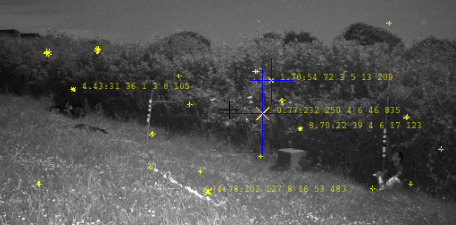
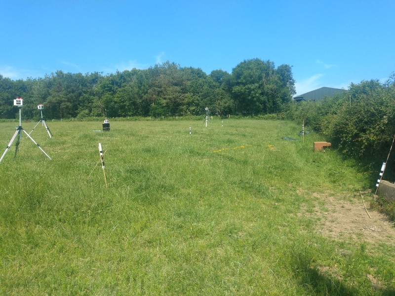
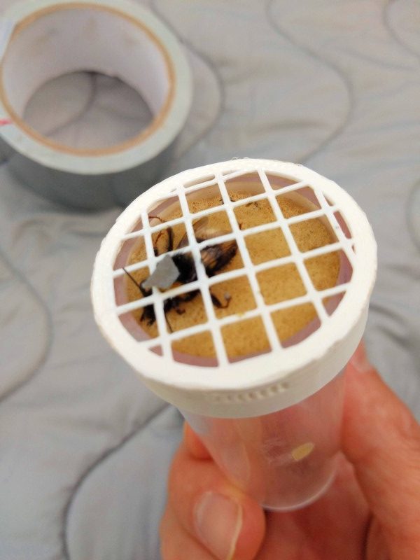
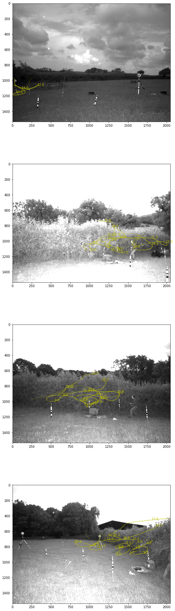
In my application however I’ve found that isn’t sufficient. My application is calibrating lots of [low cost] air pollution sensors scattered across a city (one or two sensors are ‘reference’ and are assumed to give correct measurements). Some sensors can move & it’s assumed when sensors are colocated they’re measuring the same thing. In my model each sensor has a transformation function (parameterised by a series of correlated random variables that have GP priors, over time) this function describes the scaling etc that the cheap sensors do to the real data. We assume these can drift over time. For now imagine this is just a ‘calibration scaling’ each sensor needs to apply to the raw signal to get the ‘true’ pollution, at a given time.

A-priori the scaling for each sensor is assumed to be independent, but once two sensors (A & B) have been in proximity their (posterior) scalings are very very correlated. If B is colocated with sensor C and C with D, etc, it will lead to very strong correlations in these scaling variables across the network. Importantly these correlations are induced by the observations and are only in the posterior, not the prior. The upshot is that the whitening provided by the prior covariance doesn’t help decorrelate the latent variables much, and I found the HMC really struggled to mix.

The Idea
I was thinking an obvious solution is to run ‘normal’ Variational Inference first, using a standard multivariate Gaussian for the approximating distribution, q(u). Then, once it’s (very) roughly optimised, use the covariance from q(u) instead of the covariance from the prior for whitening. This way we hopefully will have the benefit of a complicated distribution provided by HMC but it can still sample/mix successfully.

[1] Blei, David M., Alp Kucukelbir, and Jon D. McAuliffe. “Variational inference: A review for statisticians.” Journal of the American statistical Association 112.518 (2017): 859-877. link

[2] Rue, Håvard, Sara Martino, and Nicolas Chopin. “Approximate Bayesian inference for latent Gaussian models by using integrated nested Laplace approximations.” Journal of the royal statistical society: Series b (statistical methodology) 71.2 (2009): 319-392. link

[3] Hensman, James, et al. “MCMC for variationally sparse Gaussian processes.” Advances in Neural Information Processing Systems. 2015. link

I’ve started looking at bumblebee flight paths (especially during initial orientation flights from the nest). To this end I’ve wanted to increase the acquisition frequency of the system.

I found that firing more frequently than about every 1.6s seconds lead to marked decreases in the actual brightness of the flash. Instead I’ve rebuilt the electronics to allow the flashes to be fired sequentially. I have previously done this but found often the flashes would end up firing together. I assumed my circuit had a short, but I found the same happened again in my new circuit. I experimented for a while adding various capacitors across the supply rail (thinking maybe there was a ‘spike’ coming back through the two trigger wires from the flash), with the same thinking I added a reversed diode across those lines to catch any such spike. None of this helped.

I eventually found that spreading the flashes out across my desk helped a lot… this wasn’t expected, and suggested the problem was likely to be electromagnetic interference. The flash going off involves considerable current*, which even given the small size of the flash probably will equate to quite a large whole-spectrum EM pulse.

After chatting with helpful people on freenode’s ##electronics, I tried out tin-foil, and found (as long as each flash & wire was wrapped in its own foil & not touching) the 4 flashes would fire independently.

I’ll try out using some household build thermal insulation tape to shield the flashes next as that will be a little more tidy. I also found direct sunlight got the black casings quite hot so they will probably benefit from the silver foil for that reason too.

*back of the envelope calculation: If the flash (at 1/32) is abour 3J over 10us (=300kW) with say, 300V across it, then the current will be on the order of 300kW/300=1kA.