Mike's Page

Informatics, Development, Cycling, Data, Travel ...

Adversarial Examples for Gaussian Processes

First, apologies for the pause in blog posts – I’ve been away on shared parental leave for the last few months with my new “project” (aka Samuel :).

Anyway, adversarial examples are now a heavily researched area of machine learning. Modern methods now exist that can successfully classify a test point in high dimensional, highly structured datasets [citation needed, such as images etc]. It has been found however that these successful classification results are susceptible to small perturbations in the location of the test point [e.g. Szegedy et al. 2013]. By carefully crafting the perturbations the attacker can cause an ML classifier to misclassify even with only a tiny perturbation. Many examples exist, from malware detection [Srndic and Laskov, 2014] to vision for autonomous vehicles [Sitawarin et al. 2018].

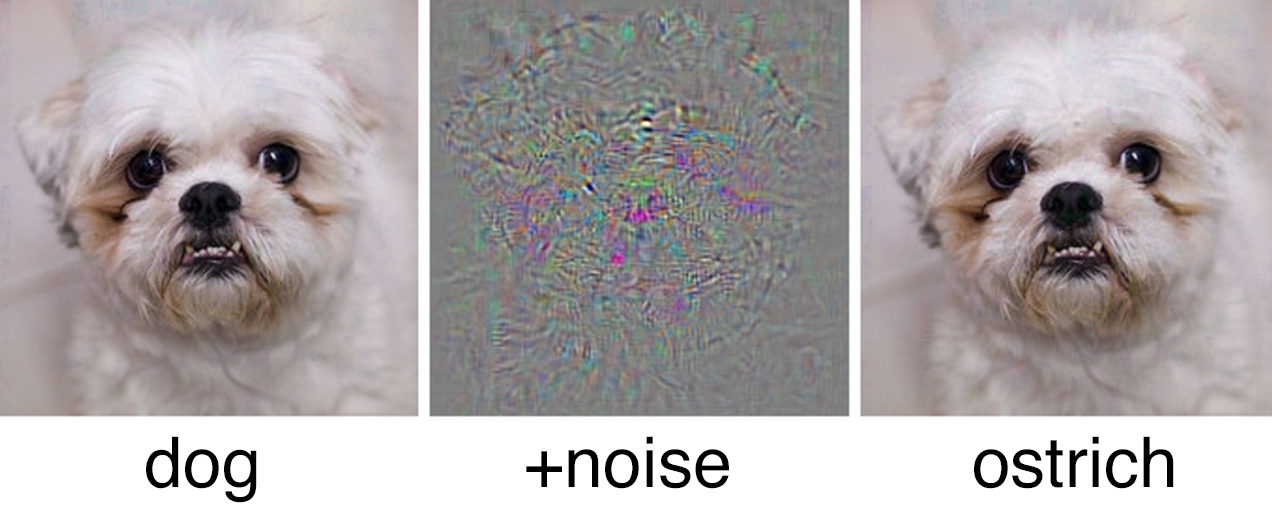
Image from Szegedy, Christian, et al.

Image from Szegedy, Christian, et al. “Intriguing properties of neural networks.” arXiv preprint arXiv:1312.6199 (2013). Tiny, carefully crafted, changes can cause a misclassification.

Typically in these papers the authors take a correctly classified training point of one class and alter it to become a different class.

A few thoughts on this;

  • First, it isn’t clear to me how close to the decision boundary the training points are, one could probably always find real examples that lie very close to the decision boundary and with a tiny tweak could be nudged over the line. I figured that it made more sense to look at examples in which one could move from a highly confident classification of one class to a highly confident classification in another. To motivate with a more practical example, if my self-driving car is only 55% confident the traffic light is green, I’d expect it to stop. It’s what happens if you can move it from 99% confident of a red light to 99% confident of a green.
  • Second, deep (convolutional) neural networks struggle with uncertainty – lots of methods have been proposed to try to allow them to quantify that uncertainty a little better, but typically they still seem to do weird things away from where the true training data lies (which is exactly the parts of the domain where adversarial samples lie).
  • Third, DNNs have no strong priors about the decision function. To demonstrate if one trains with a low dimensional training set, in which the classes are very separable, the decision boundary provided by the DNN is often close to one of the classes, and is often very sharp.
  • A Gaussian process classifier however has strong priors on its latent function, leading to slow changes to the classification. Hence to move between one confident location to another typically requires a large change in the training location.

My collaborators at CISPA (Saarland, Germany) are busy looking at the empirical improvements one can acheive using GPs. I thought it might be interesting to focus on whether one can bound the impact of an adversarial example.

There are typically two ways of generating adversarial examples, the first (illustrated by the dog/ostrich example) involves making small changes to lots of inputs. The second involves modifying a few inputs a lot. In the paper I’m drafting at the moment this is the path I have taken. The question: Can I produce an upper bound on the change in the latent function (or even better in the classification) that changing D inputs could cause?

So for example, if you have a GP classifier distinguishing between two digit image types, how much could the class change if you alter (say) three pixels?

I approached this problem as follows;

  • First I restricted the type of kernel to the RBF (EQ) kernel.
  • I then consider the change that can occur due to each training input (considering the output as the sum of a set of Gaussians – using the representer theorem).
  • I devised a method for bounding the sum of a mixture of Gaussians.
  • There’s a bunch of other optimisations etc to achieve a better bound.

Currently I’m just trying this out on some example training data (MNIST!), I suspect that it will only work on low dimensional problems (e.g. less than 20 dimensions) as above that the domain still is too large to search.

Ethics and Algorithms

Popular discourse around “AI” has recently particularly focused on the issue of ethics in the algorithm. Examples include the issue of discrimination (maybe when deciding whether to give someone credit or select the insurance premium), or when making split-second decisions around whether a self-driving vehicle should dodge an oncoming car by veering into a pedestrian.

My suspicion is that many of these issues are already in algorithms that we use every day, but that we don’t call “artificially intelligent”.

First, I’ll briefly consider the issue of discrimination; to reiterate the general consensus that it isn’t the algorithm that’s bias, but rather the data that it learns from. A recent example was that ethnic minorities pay a ‘penalty’for their car insurance. I briefly looked at the analysis, and I suspect (but haven’t tested) that the difference may be due to the region where different demographics live. Minority ethnic groups are more likely to live in cities, where there is more vehicle crime, hence the apparent ‘ethnic penalty’.

What do we do about this? Without looking into what latent variables explain the difference one might simply correct for the difference by adjusting the premium to ensure that the sensitive variable (race) is no longer correlated with price. However this ends up with new biases (potentially associated with variables that are unrecorded by the researcher/company). Personally I also worry that current attempts to correct biases, e.g. in recruitment could unwittingly discriminate against subpopulations that we aren’t measuring or detecting.

Second, life-and-death decisions are already being taken ‘automatically’ by algorithms. I was recently emailed by someone asking for examples of “near-term, real-life situations where AI will have to make unsupervised ethical choices…for the developing world.” Already in clinic machines are providing decision support assistance to doctors and consultants when diagnosing or prescribing treatment.

A very simple example from a developing country, can be found on the nutrition unit of Mulago Hospital, Uganda. There mothers arriving with malnourished children and the children are assessed for treatment. This can be as simple as measuring their middle-upper-arm circumference (MUAC) and comparing it to a given threshold to decide whether the child has Severe Acute Malnutrition (SAM) and thus will receive treatment. The nutritionists on the ward will also take into account other aspects of the child’s health (HIV, oedema, etc), but, in effect we are already following an algorithm.

These algorithms have been developed through scientific observational studies, investigating the outcomes of children with different MUAC.

How is machine AI different? Foremost is the opacity in the decision making. In principle the process is similar – the machine has observed lots of training examples, and has to make a decision about whether a child needs treatment. Unlike the human-implemented case, the exact reasons for a decision may be unclear.

For the last few years there has been considerable debate about the importance of interpretability, and concerns around the fragility of deep learning (in particular with respect to Adversarial Examples and the apparent sensitivity of the networks to changes in the source distribution. Arguably it is unclear, from the practitioners point of view, why a given threshold is used even in the human-algorithm case.

In summary, we are already letting algorithms make life-or-death decisions, potentially without fulling understanding the rationale behind a threshold. The process at the moment is simple, as the dimensionality of the data increases the reasoning becomes increasingly opaque, and maybe it is this that raises concern around AI making such decisions?

Bumblebee May 2018 Update

First flight

Last week we flew the bumblebee tracker for the first time.

It was really useful having lots of volunteers helping out!

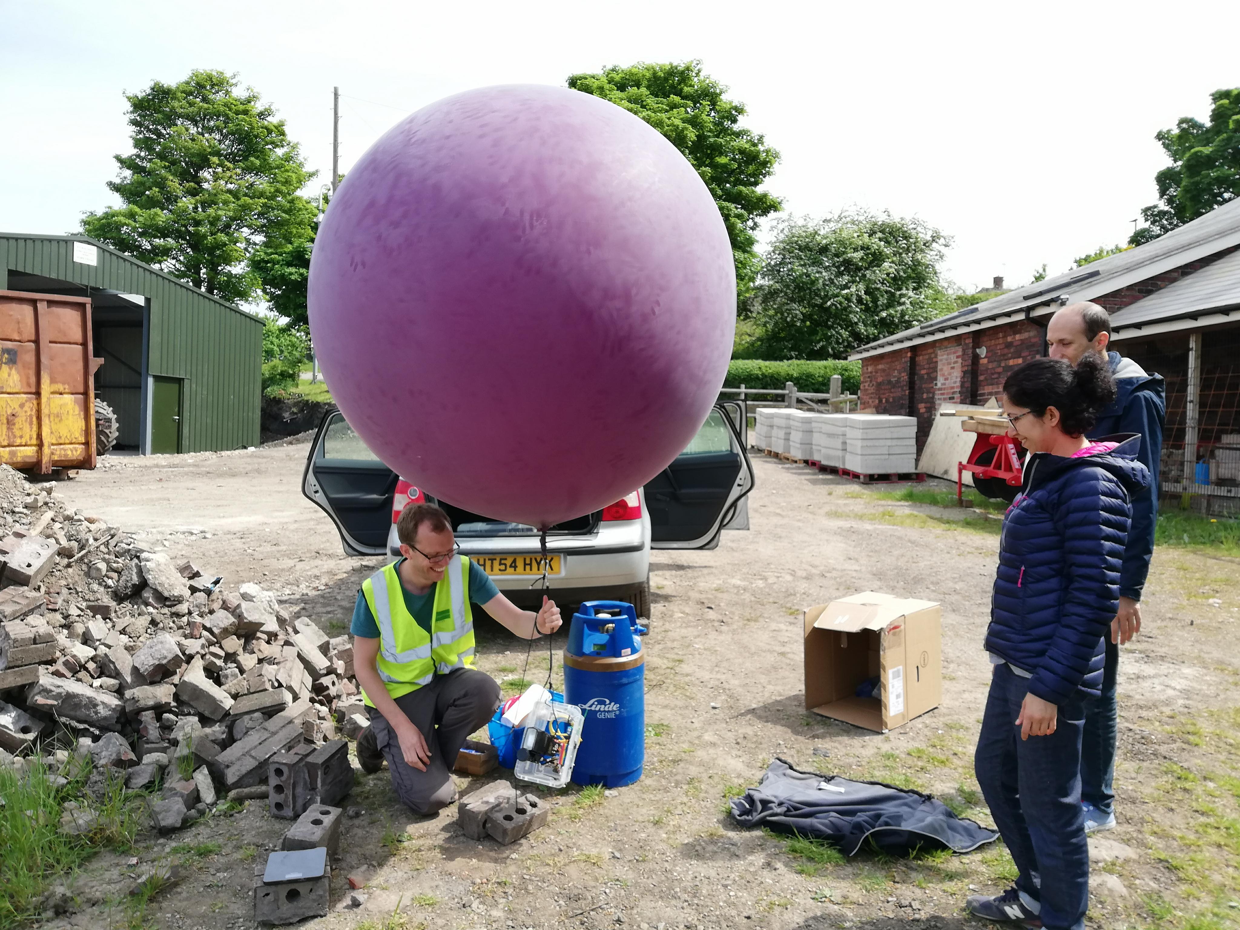
Everyone helped fill the balloon!

Everyone helped fill the balloon!

It was surprisingly easy to get the balloon in the air, but the slightest gust did cause quite a bit of movement.

Balloon in flight (taken by Mike Livingstone)

Balloon in flight (taken by Mike Livingstone)

We successfully tracked the retroreflector from about 20m up. I need to make the software quicker.

Second flight

Today (28th May) we tested the bumblebee experiment again. It was almost the same as a test two weeks ago but the reflector used was slightly larger than before (about 0.9 cm2) and we used a filter. Again we tested the system by tracking a reflector attached to a string.

Filter

The ground and plants reflect relatively little UV and visible-violet spectrum. So we added to the camera a 390nm bandpass filter, that ranges from about 335nm [near UV] to 445nm [violet/deep-blue]. This had the effect of filtering out much of the background leaving the reflections from the camera flash/retroreflector.

We tested the system by moving the reflector on the end of a black string along the length of the site, to see if the system could identify its location.

Demonstration of tracking reflector from balloon mounted system

Demonstration of tracking reflector from balloon mounted system. Actual location marked with yellow circle. The identified location is marked with a white cross. The confidence in the identification is written in the title. Photos 5 seconds apart. Exposure: 2ms, Gain 30dB, blocksize/step/offset: 20/10/3.

We were able to track the fake-bee successfully – probably from about 30m high. I think it’ll work considerably higher, unfortunately we’ve not tested it that high yet. 30m feels suddenly really high when you’re looking up at it!

Balloon connection failure

The experiment came to an abrupt end when the balloon rubber loop failed, causing the hardware to fall and crash catastrophically. The balloon escaped.

I’d followed these instructions from public lab. However the single-rubber-loop wasn’t sufficient and failed.

Single rubber loop problem

Single rubber loop problem

The crashed system:

Remains for the crashed experiment!

Remains of the crashed experiment!

Lessons

  • The filter seems to help a lot!
  • The retroreflective paint doesn’t work
  • Three tethers is more stable than two

Most important are safety lessons around the fallen experiment:

  • Double-up the rubber hoops
  • Add a parachute
  • Wear hard-hats
  • Place an exclusion zone – during the experiment
  • Make it lighter

Next steps

  • Build new lighter version
  • Test if we can stick things to insects (get the hang of this before we fly again)

Coregionalised Air

Air pollution coregionalised between the US embassy and Makerere campus

Air pollution coregionalised between the US embassy and Makerere campus

Next week I’ll be presenting at Manchester’s Advances in Data Science conference, on the air pollution project. I’ve written an extended abstract on the topic.

We use a custom-crafted kernel for coregionalising between multiple sensors, to allow us to make probabilistic predictions at the level of the high-quality reference sensor, across the whole city, using the low-quality noisy sensors. We estimate the coregionalision parameters using training data we’ve collect – which ideally should include close or colocated measurements from pairings of sensors.

In future we hope to:

  1. Include the uncertainty in the coregionalisation (e.g. by integrating over the distribution of the coregionalisation parameters, e.g. using CCD.
  2. Allow this coregionalisation to vary over time. This will require non-stationarity, and is probably best achieved using a more flexible, non-analytic solution. E.g. writing the model in STAN
  3. .

  4. Updating the model in real time. I think another advantage of using a STAN or similar framework would be the gradual inclusion of new MC steps incorporting new data, as we throw out old data, this allows the gradual change of coregionalisation to be incorporated.

Update

Building flat coregionalisation kernel

Building flat coregionalisation kernel

We can’t just use the standard coregionalisation kernel, as we’re not just kronecker-product multiplying a coregionalisation matrix with a repeating covariance matrix. Instead we want to element-wise multiply a matrix that expresses the coregionalisation with another matrix that expresses the covariance due to space and time proximity (see above figure).

Here is the GPy kernel code to do this;

import GPy
import numpy as np
from GPy.kern import Kern
from GPy.core.parameterization import Param
#from paramz.transformations import Logexp
#import math
class FlatCoreg(Kern): 
    """
    """

    def __init__(self, input_dim, active_dims=0, rank=1, output_dim=None, name='flatcoreg'):
        super(FlatCoreg, self).__init__(input_dim, active_dims, name)

        assert isinstance(active_dims,int), "Can only use one dimension"
        
        
        W = 0.5*np.random.randn(rank,output_dim)/np.sqrt(rank)
        self.W = Param('W', W)
        self.link_parameters(self.W) #this just takes a list of parameters we need to optimise.

    def update_gradients_full(self, dL_dK, X, X2=None):
        
        if X2 is None:
            X2 = X.copy()
            
        dK_dW = np.zeros([self.W.shape[1],X.shape[0],X2.shape[0]])
        for i,x in enumerate(X):
            for j,x2 in enumerate(X2):
                wi = int(x[0])
                wj = int(x2[0])
                dK_dW[wi,i,j] = self.W[0,wj]
                dK_dW[wj,i,j] += self.W[0,wi]
        self.W.gradient = np.sum(dK_dW * dL_dK,(1,2))
       

    def k_xx(X,X2,W,l_time=2.0,l_dist=0.1):
        #k_time = np.exp(-(X[0]-X2[0])**2/(2*l_time))
        #k_dist = np.exp(-(X[1]-X2[1])**2/(2*l_dist))
        k_coreg = coregmat[int(X[2]),int(X2[2])]
        return k_coreg #k_time * k_dist * k_coreg 
        
    def K(self, X, X2=None):
        coregmat = np.array(self.W.T @ self.W)
        if X2 is None:
            X2 = X
        K_xx = np.zeros([X.shape[0],X2.shape[0]])
        for i,x in enumerate(X):
            for j,x2 in enumerate(X2):
                K_xx[i,j] = coregmat[int(x[0]),int(x2[0])]
        return K_xx
    

    def Kdiag(self, X):
        return np.diag(self.K(X))

k = (GPy.kern.RBF(1,active_dims=[0],name='time')*GPy.kern.RBF(1,active_dims=[1],name='space'))*FlatCoreg(1,output_dim=3,active_dims=2,rank=1)
#k = FlatCoreg(1,output_dim=3,active_dims=2,rank=1)
#k.coregion.kappa.fix(0)   

This allows us to make predictions over the whole space in the region of the high quality sensor, with automatic calibration via the W vector.

DASK and ec2 – use daskec2lite

I’ve started having the same problem as in this issue. I think something else has been updated which has caused the new error. As it says on the dask-ec2 readme, dask-ec2’s project is now deprecated – and so I didn’t try fixing the new bug. I tried for a while using kubernetes (kops, terraform, etc), but it’s quite a pain to set up (not well documented yet maybe) and is serious overkill for what I want (and probably what a lot of people want…). So instead…

I’ve written a replacement for dask-ec2, I’ve called daskec2lite.

It needs a little bit more work but is nearly finished. I’ll hopefully have some time later in the year to get it to a more ‘release’ state, but feel free to use it.

daskec2lite --help

usage: daskec2lite [-h] [--pathtokeyfile [PATHTOKEYFILE]]
[--keyname [KEYNAME]] [--username [USERNAME]]
[--numinstances [NUM_INSTANCES]]
[--instancetype [INSTANCE_TYPE]] [--imageid [IMAGEID]]
[--spotprice [SPOTPRICE]] [--region [REGION_NAME]]
[--wpi [WORKERS_PER_INSTANCE]] [--sgid [SGID]] [--destroy]

Create an EC2 spot-price cluster, populate with a dask scheduler and workers.
Example: daskec2lite --pathtokeyfile '/home/mike/.ssh/research.pem' --keyname
'research' --username 'mike' --imageid ami-19a58760 --sgid sg-9146afe9

optional arguments:
-h, --help show this help message and exit
--pathtokeyfile [PATHTOKEYFILE]
path to keyfile [required]
--keyname [KEYNAME] key name to use to access instances [required]
--username [USERNAME]
user to log into remote instances as [required]
--numinstances [NUM_INSTANCES]
number of instances to start
--instancetype [INSTANCE_TYPE]
type of instance to request
--imageid [IMAGEID] AWS image to use [required]
--spotprice [SPOTPRICE]
Spot price limit ($/hour/instance)
--region [REGION_NAME]
Region to use
--wpi [WORKERS_PER_INSTANCE]
Workers per instance
--sgid [SGID] Security Group ID [required]
--destroy Destroy the cluster

Bumblebee Tracking

Outside of my university work, building a bumblebee tracking system is my main hobby ‘research’ project. A snippet from a draft paper,

Researchers studying bumblebees currently are unable to track the bee’s movement outside the nest without the use of prohibitively expensive radar tracking systems (Goulson 2003) which, besides their cost, have limited range and only work for flat landscapes with few obstructions. Proxies for bee tracking include mark and recapture to estimate their range, although this is often bias by the location of the observers (Schaffer 1996).

An ability to track bumblebees has three important benefits: Firstly it gives conservationists valuable information regarding foraging and mating range and behaviour, which will inform habitat management (for example in avoiding fragmentation). Secondly, it allows researchers to tag and then follow workers back to the nest, allowing the nests of rare species to be found and studied. In particular the recent reintroduction of Bombus subterraneus would greatly benefit from such a technology, which would allow researchers to count nests and inspect them for indicators of reproductive success and provide insight into the habitats most suitable for nest building in this species. Thirdly, the method could be combined with other experiments, such as the ongoing investigations into the effect of neonicotinoid exposure on navigation.

Hypothesis

Can an aerial camera combined with retroreflective tags track bumblebees?

Method

A compact camera and flash are mounted (with control electronics) on an tethered balloon platform, approximately 100m above the ground. A retroreflective material is attached to the back of the bumblebee to be tracked. Every 2-5 seconds two photos are taken (with and without the flash). A short exposure time (1/1000s) is used, made possible by the in-lens shutter in the compact camera. The retroreflective patch on the bee reflects the flash’s light back towards the camera, causing the reflector to appear as a bright spot against a relatively dark background. The images are sent to a laptop on the ground (via a raspberry pi and wifi) where software (python) aligns the two images and then subtracts them. The retroreflective dot is revealed as the brightest point in the image, which is automatically identified.


Progress & Development

2015: Version 1

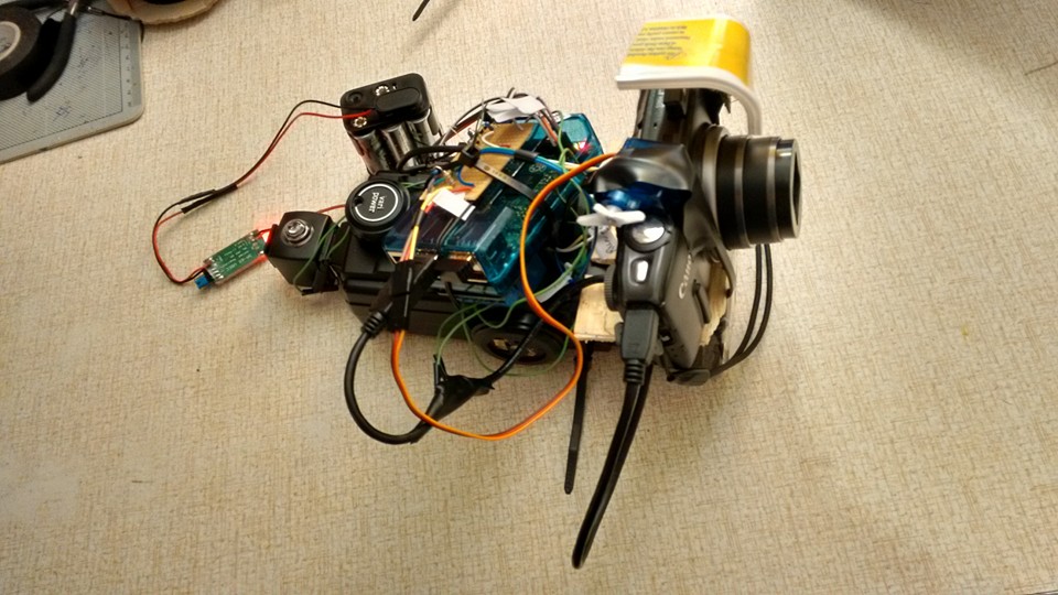
I started with a compact camera. To make this work I needed a servo to press the trigger and a pair of relays to connect/disconnect the USB and the flash to the camera (by disconnecting the USB the camera went into shooting mode, reconnecting allowed me to copy the images).

Version 1 - with compact camera

Version 1 – with compact camera

2016: Dalliance with Drones

I tried for a while to get the thing lifted by a drone, but it’s quite heavy, and the drone is an additional hassle (with limited air time, etc). After much faffing about with them I decided to switch back to a tethered balloon.

2017: Version 2; better camera & software

Thanks to a second grant from the Socially Enterprising Researcher grant, here at the university of Sheffield, I was able to buy a smartek gcc2062m camera (which can be triggered with a high to a pin), and has an electronic shutter.

I next developed two python software components;

  • A module to locate the retroreflector in a pair of images.
  • A module to control the camera data, the camera trigger, the detection algorithm and a web interface to the system.
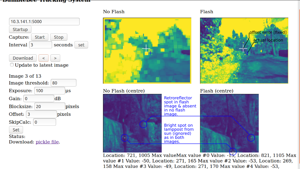
Here's a screenshot of an earlier version.

Here’s a screenshot of an earlier version.

2018: Testing

An initial test of the new system, over a distance of about 23m worked very well. However the range tested needs increasing, and a smaller retroreflector needs testing (currently it’s 1cm^2).

I also want to add code that filters the retrodetection image to find only peaks (rather than other structures). Later I’ll include a particle filter to track the target between images. Currently each image is processed separately.

Twentry images showing retroreflector being tracked: First 9 images - reflector was attached to hedge at + mark. Following 7 images, I carry it across the image. One image it's placed on the ground, with the last two attached ontop of the hedge.

Twentry images showing retroreflector being tracked: First 9 images – reflector was attached to hedge at + mark. Following 7 images, I carry it across the image. One image it’s placed on the ground, with the last two attached ontop of the hedge.

Version 2: With new camera, flash, and no relays or servos.

Version 2: With new camera, flash, and no relays or servos.

Smoking flash

I tried testing a greater range, but unfortunately the flash experienced a catastrophic failure and started smoking… I’ll buy a new flash and report back!

Update

With a new flash things are working well again. I had trouble with ensuring that it is well focused, so have added a few more controls to the interface to see a ‘zoomed in’ central part of the image:

Latest Interface

Latest Interface. Click for full-size image.

The above test was from about 40m. We’ll soon test at 80m.

I’ve also ordered a canister of helium (£118!) to collect next Monday. And hopefully will be testing it out on a balloon in the next few weeks.

Using Numba

Numba lets you JIT (just in time) compile chunks of python down to machine-code-speeds. In theory it’s as simple as adding the @jit decorator to your methods, in practice it’s a bit more complicated!

Just a few things I’m finding while trying to convert my code to work with numba. In particular it turns out it’s better to think about numba in advance, rather than try to convert old code to work with it (I think)…

  • Returning more than one variable (in a tuple). From stackoverflow, we have the useful nb.typeof() hint;

    @nb.jit(nb.typeof((1.0,1.0))(nb.double),nopython=True)

  • Tuples are more likely to work than lists, and numpy arrays seem robust too. Basically don’t start nesting lists.

A space elevator without needing magic materials

Model of the partial space elevator (start height=3000km,

Model of the partial space elevator

You are probably familiar with the idea of a space elevator; a rope extending from the Earth’s surface to beyond geostationary (with a counterweight attached). This has the amazing property that one could just ‘climb’ the rope. The counterweight pulls the rope back on station even. The kinetic energy gained by the payload comes at the cost of slowing the Earth’s rotation slightly. Brilliant. The problem with this is that to make the rope, one needs unobtainable materials. Huge amounts of carbon nanotubes or something.

There’s bound to be good reasons the following suggestion wouldn’t work. But I’m curious what they are. Rather than start on the Earth’s surface, what if our elevator starts at 2000km above the surface? This will allow us to build the rope out of much more reasonable materials. Why? The original rope needs to be strong as there’s a lot of it being pulled towards the Earth (and more being pulled the other way by the counter-weight). To hold this stuff up requires a lot of material, which is heavy, which means we need even more material, etc. Also the force of gravity is stronger closer to the Earth!

“How’s it stay up?” You might reasonably ask. This elevator, unlike the last is in ‘proper orbit’, or at least it is, on average. The part that hangs towards the Earth will be suborbital (indeed will be going quite slowly relative to low-earth orbit).

“But how do we get to the start of the tether if it’s 2000km up?” Going up into space is easy, getting into orbit is the expensive bit. An (awfully named) rockoon might be a neat way to get to the 2000km mark with a very modest rocket (the rocket equation means that we can use a very small rocket to get to 2000km, compared to the rocket required to get to 2000km orbit).

“But won’t you pull the whole thing down as you climb it?” Yes. To correct for this, ion-engines will be arranged on the tether for station-keeping. Some of the payload can be used for refuelling these (they have a specific impulse 10-100 times better than a rocket launcher so hopefully we’ll need less fuel!)

Some rough calculations

This one only is as high as geostationary, it is actually going faster than geostationary orbit (at that, and all altitudes).

Here I don’t allow for any extra forces or weakness, and assume we have available the full 5.8GPa strength of Zylon. Hopefully newer materials that are appearing that combine nanotubes and polymers will allow this assumption! Next I assume we can get to 2000km above the Earth with a rockoon. If I’ve applied the rocket equation correctly I think we’d need 2kg of fuel for each kg of payload etc (and some of that payload has to be propellant for the ion-engines on the tether). Still not bad though. If our materials improve we could get the start closer to the Earth. Anyway; this tether will be about 1cm wide at its widest point, and weigh about 2100 tonnes (the new Falcon Heavy can lift 26.7tonnes to GTO), if 2/3rd of that payload is tether, we’d need 118 flights (or less as we could start using the tether for the bottom part!).

Update

Asked the question on stackexchange. Still can’t find any papers etc on this particular idea. In response to one of the questions on SE I ran a few more simulations – interestingly unstable, but I wonder if this instability can be mitigated by adjusting the length of the tether!

Christmas Squirrel

Christmas Squirrel

Christmas Squirrel


This year I made my mum a Christmas Squirrel!

What it does:

Give it one of the small Christmas things or birds and it will play a Christmas song or a radio station (4, classic or 3).

It uses an RFID reader, an audio amp and some other gubbins. It uses a raspberry pi and uses internet radio to get the audio streams.

The git repo is here: https://github.com/lionfish0/christmas_squirrel.

The volume control is a large circular button on its back.

I’ll try to get some photos when I next see it!

Using DASK with EC2 for embarrassingly parallel problems

Update 3

kubernetes is too complicated. Instead I’ve written a replacement for dask-ec2, I’ve called daskec2lite. See new post.

Update 2

DASK EC2 has been deprecated. It is now recommended people use kubernetes. I’ve not experimented with this yet.

Update 1

pip was upgraded to 9.0.2 a few days ago, which has caused problems. Basically the error message people will get when using dask-ec2 will be of the form "pip.installed' is not available".

I fixed this in dask by making two changes:

  • To line 167 in salt.py, I specified that I wanted the older version of pip installed (added 9.0.1 to the string): pip==9.0.1.
  • Line 48 in formulas/salt/dask/distributed/init.sls I removed a reference (I think I added originally!) to python36-pip and just used python3-pip.

This version of dask-ec2 is on github.

DASK

DASK is a library (for python) which lets you distribute computation over a cluster. DASK_EC2 is another module (closely related) which allows you to use AWS EC2 framework for creating the cluster etc. Just a quick note: DASK is good if your problem is embarrassingly parallel. Examples I’ve come across regularly, include:

  • Cross-validation
  • Fitting multiple datasets (e.g. separate patients)
  • Parameter-grid search

I’ve found that DASK_ec2 isn’t being maintained at the moment, so I’ve made a repo with some of the changes I’ve needed here. The changes I’ve incorporated:

1. Allowing the use of spot-instances (see https://github.com/dask/dask-ec2/pull/66)
2. Fixed a bug to allow the distributed computers to use 16.04 (see https://github.com/dask/dask-ec2/issues/98)
3. Version of anaconda being downloaded was out of date (see https://github.com/dask/dask-ec2/issues/38 and https://github.com/dask/dask-ec2/compare/master…lionfish0:master#diff-a7ee77124863ef31e39bc6f1673632c8)

How to install

Get AWS setup

From https://boto3.readthedocs.io/en/latest/guide/quickstart.html (Boto is the Amazon Web Services (AWS) SDK for Python)

sudo apt-get install awscli
pip install boto3

Visit AWS -> IAM -> Add user -> Security Credentials -> Create Access Key. Run aws configure and enter the ID, code, region. Notes, I use for region ‘eu-west-1’, outputformat is blank (leave as JSON).

Test

Try this python code and see if it works.

import boto3
s3 = boto3.resource('s3')
for b in s3.buckets.all():
    print(b.name)

From http://distributed.readthedocs.io/en/latest/ec2.html, it says to install dask-ec2 with pip install dask-ec2 (don’t do this!!!) instead now get from my repo with the above changes incorporated:

pip install git+https://github.com/lionfish0/dask-ec2.git

Sort out keys

Visit AWS->EC2->Key pairs->Create key pair. I called mine “research”. Save the keyfile in .ssh, chmod 600.

Select AMI (instance image we want to use)

Get the AMI we want to use (e.g. ubuntu 16.04). Check https://cloud-images.ubuntu.com/locator/ec2/ and search for e.g. 16.04 LTS eu-west-1 ebs.

Edit: It needs to be an hvm, ebs instance. So I searched for: “eu-west-1 16.04 ebs hvm”.

To start up your cluster on EC2

We can start up the cluster with dask-ec2 but it wants some parameters, including the keyname and keypair. I found I had to also specify the region-name, the ami and tags as the first two have wrong defaults and the tool seems to fail if tags isn’t set either. Also found using ubuntu 16.04 had a SSL wrong version number error which is fixed hopefully if you use my version of the dask-ec2 repo (see https://github.com/dask/dask-ec2/issues/38 ). count specifies the number of on-demand instances (has to be at least 1 at the moment). spot-count is the number of spot instances (combine with the spot-price, which I set to the price of the on-demand instances). The volume-size is the size in Gb of the instance hard disk, and the type is the ec2 instance type. The nprocs is the number of calculations the computer will be given to work with I think. As GPy does a good job at distributing over multiple cores, I just give each instance 2 problems at a time.

dask-ec2 up --keyname research --keypair .ssh/research.pem --region-name eu-west-1 --ami ami-c8b51fb1 --tags research:dp --count 1 --spot-count 5 --spot-price 0.796 --volume-size 10 --type c4.4xlarge --nprocs 2

Eventually after a long time, this will finish with:

Dask.Distributed Installation succeeded
Addresses
---------
Web Interface:    http://54.246.253.159:8787/status
TCP Interface:           54.246.253.159:8786
 
To connect from the cluster
---------------------------
dask-ec2 ssh  # ssh into head node
ipython  # start ipython shell

from dask.distributed import Client, progress
c = Client('127.0.0.1:8786')  # Connect to scheduler running on the head node
 
To connect locally
------------------
Note: this requires you to have identical environments on your local machine and cluster.
 
ipython  # start ipython shell
 
from dask.distributed import Client, progress
e = Client('54.246.253.159:8786')  # Connect to scheduler running on the head node
 
To destroy
----------
 
dask-ec2 destroy
Installing Jupyter notebook on the head node
DEBUG: Uploading file /tmp/tmp1GOH7d to /tmp/.__tmp_copy
DEBUG: Running command sudo -S bash -c 'cp -rf /tmp/.__tmp_copy /srv/pillar/jupyter.sls' on '54.246.253.159'
DEBUG: Running command sudo -S bash -c 'rm -rf /tmp/.__tmp_copy' on '54.246.253.159'
+---------+----------------------+-----------------+
| Node ID | # Successful actions | # Failed action |
+=========+======================+=================+
| node-0  | 17                   | 0               |
+---------+----------------------+-----------------+
Jupyter notebook available at http://54.246.253.159:8888/ 
Login with password: jupyter

Install libraries on cluster

Importantly the remote cluster’s environments have to match the local environment (the version of linux, the modules, the python version, etc all have to match). This is a bit awkward. Finding modules is a problem…I found these not to work out the box. Critically, it failed with “distributed.utils - ERROR - No module named dask_searchcv.methods“. I found I had to intstall the module on each worker:

Either by hand:

local$ dask-ec2 ssh 1
dask1$ conda install dask-searchcv -c conda-forge -y

Or better is to write a python function to do this for us – I run this every time I startup a new cluster, to install all the stuff I know I need.

def install_libraries_on_workers(url):
    """Install libraries if necessary on workers etc.
    
    e.g. if already on server...
    install_libraries_on_workers('127.0.0.1:8786')
    """
    from dask.distributed import Client
    client = Client(url)

    runlist = ['pip install -U pip','sudo apt install libgl1-mesa-glx -y','conda update scipy -y','pip install git+https://github.com/sods/paramz.git','pip install git+https://github.com/SheffieldML/GPy.git','pip install git+https://github.com/lionfish0/dp4gp.git','conda install dask-searchcv -c conda-forge -y', 'pip install git+https://github.com/lionfish0/dask_dp4gp.git', 'pip install numpy', 'conda remove argcomplete -y']#, 'conda install python=3.6 -y']

    for item in runlist:
        print("Installing '%s' on workers..." % item)
        client.run(os.system,item)
        print("Installing '%s' on scheduler..." % item)
        client.run_on_scheduler(os.system,item)    
        #os.system(item) #if you need to install it locally too

Example

Here’s a toy example to demonstrate how to use DASK with GPy

import numpy as np
import matplotlib.pyplot as plt
%matplotlib inline
import GPy
from dask import compute, delayed
from dask.distributed import Client

#adding the delayed line means this won't run immediately when called.
@delayed(pure=True)
def predict(X,Y,Xtest):
    m = GPy.models.GPRegression(X,Y)
    m.optimize()
    predmean, predvar = m.predict(Xtest)
    return predmean[0,0]
    #return np.mean(Y)

values = [np.NaN]*1000
for i in range(1000):
    X = np.arange(0,100)[:,None]
    Y = np.sin(X)+np.random.randn(X.shape[0],1)+X
    Xtest = X[-1:,:]+1
    values[i] = predict(X,Y,Xtest) #this doesn't run straight away!
    
client = Client(ip+':8786')

#here is when we actually run the stuff, on the cloud.
results = compute(*values, get=client.get)

print(results)

On two 16-core computers on AWS, I found this sped up by 59% (130s down to 53s).

More examples etc is available at http://dask.pydata.org/en/latest/use-cases.html

Update

If you did this a while ago, dask and things can get out of date on your local machine. It’s a pain trying to keep it all in sync. One handy command;

conda install -c conda-forge distributed

E.g.

mike@atlas:~$ conda install -c conda-forge distributed
Fetching package metadata .............
Solving package specifications: .

Package plan for installation in environment /home/mike/anaconda3:

The following packages will be UPDATED:

dask: 0.15.4-py36h31fc154_0 --> 0.16.1-py_0 conda-forge
dask-core: 0.15.4-py36h7045e13_0 --> 0.16.1-py_0 conda-forge
distributed: 1.19.1-py36h25f3894_0 --> 1.20.2-py36_0 conda-forge

The following packages will be SUPERSEDED by a higher-priority channel:

conda-env: 2.6.0-h36134e3_1 --> 2.6.0-0 conda-forge

Proceed ([y]/n)? y

dask-core-0.16 100% |################################| Time: 0:00:01 269.93 kB/s
distributed-1. 100% |################################| Time: 0:00:01 597.96 kB/s
dask-0.16.1-py 100% |################################| Time: 0:00:00 1.16 MB/s
« Older posts

© 2019 Mike's Page

Theme by Anders NorenUp ↑