First flight
Last week we flew the bumblebee tracker for the first time.
It was really useful having lots of volunteers helping out!
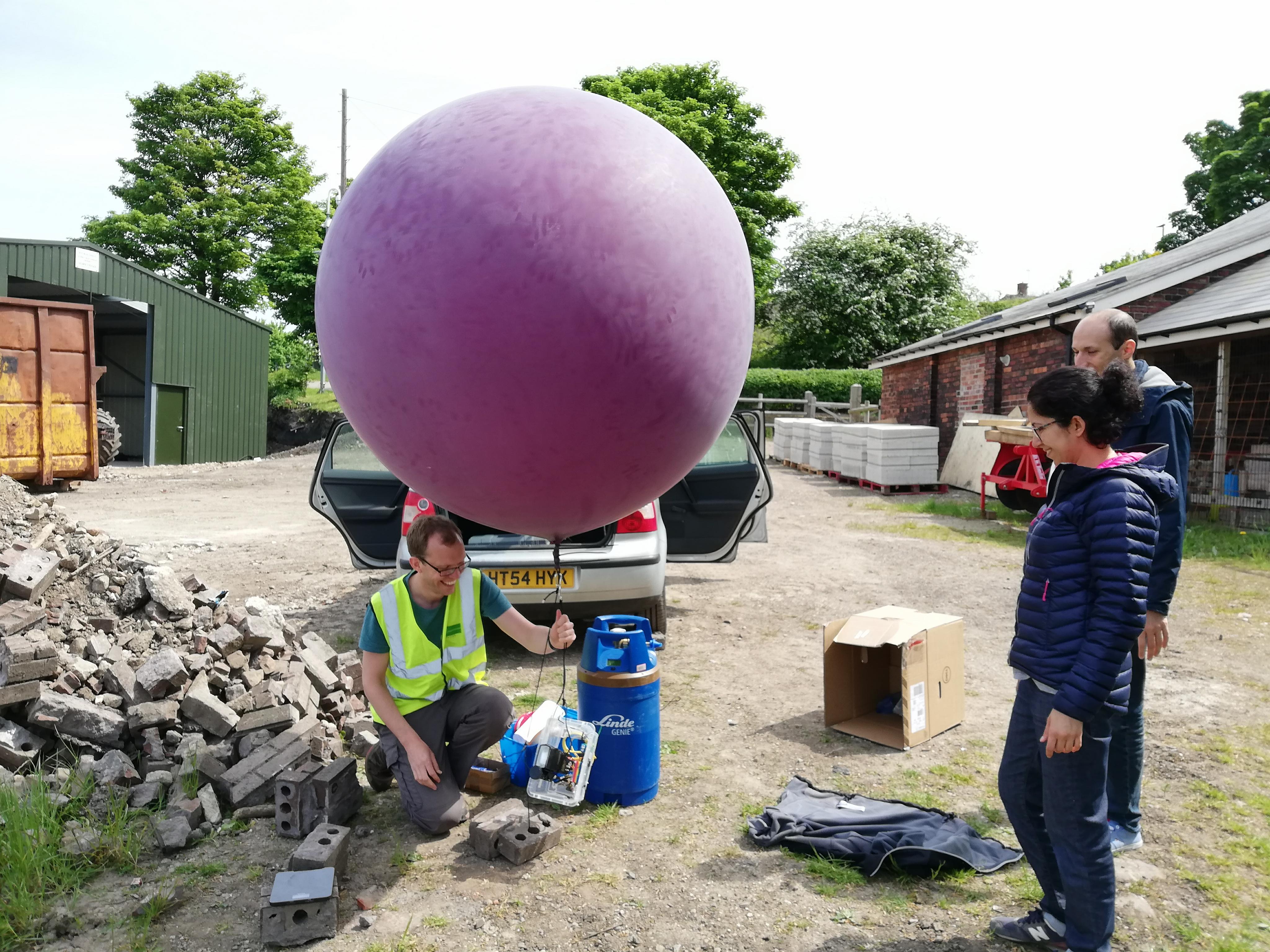
Everyone helped fill the balloon!
It was surprisingly easy to get the balloon in the air, but the slightest gust did cause quite a bit of movement.

Balloon in flight (taken by Mike Livingstone)
We successfully tracked the retroreflector from about 20m up. I need to make the software quicker.
Second flight
Today (28th May) we tested the bumblebee experiment again. It was almost the same as a test two weeks ago but the reflector used was slightly larger than before (about 0.9 cm2) and we used a filter. Again we tested the system by tracking a reflector attached to a string.
Filter
The ground and plants reflect relatively little UV and visible-violet spectrum. So we added to the camera a 390nm bandpass filter, that ranges from about 335nm [near UV] to 445nm [violet/deep-blue]. This had the effect of filtering out much of the background leaving the reflections from the camera flash/retroreflector.
We tested the system by moving the reflector on the end of a black string along the length of the site, to see if the system could identify its location.

Demonstration of tracking reflector from balloon mounted system. Actual location marked with yellow circle. The identified location is marked with a white cross. The confidence in the identification is written in the title. Photos 5 seconds apart. Exposure: 2ms, Gain 30dB, blocksize/step/offset: 20/10/3.
We were able to track the fake-bee successfully – probably from about 30m high. I think it’ll work considerably higher, unfortunately we’ve not tested it that high yet. 30m feels suddenly really high when you’re looking up at it!
Balloon connection failure
The experiment came to an abrupt end when the balloon rubber loop failed, causing the hardware to fall and crash catastrophically. The balloon escaped.
I’d followed these instructions from public lab. However the single-rubber-loop wasn’t sufficient and failed.

Single rubber loop problem
The crashed system:

Remains of the crashed experiment!
Lessons
- The filter seems to help a lot!
- The retroreflective paint doesn’t work
- Three tethers is more stable than two
Most important are safety lessons around the fallen experiment:
- Double-up the rubber hoops
- Add a parachute
- Wear hard-hats
- Place an exclusion zone – during the experiment
- Make it lighter
Next steps
- Build new lighter version
- Test if we can stick things to insects (get the hang of this before we fly again)